Transformers XAI - Understand the basics of the state-of-the-art
Transformers?
If you ask what is a Transformer, in general, people will easily define a car that becomes a killer machine (or something like this).
However, in the NLP field a Transformer is not even close to any car, or any killer, nor anything like this.
In 2017, Google introduced to the world Attention is all you need, the paper that would not only change the meaning of what is a Transformer, but also revolutionize
and improve the results of natural language tasks until the moment.
Why?
State-of-the-art
The paper achieved never seen before results in the field, improving all the previous performances previously reached.
It combined some of the best approaches until then: a seq-to-seq model, attention mechanisms and Encoder-Decoder architectures.
Simplicity
Up until that moment, the best approaches used a great variety of complex methods and architectures to achieve
good results. Convolutional Neural Networks (CNNs), Recurrent Neural Networks (RNNs) like LSTMs, etc.
Attention
The attention mechanism allows the Neural Network to understand the sequence of words in a similar way humans do,
permitting distinction between relevant and irrelevant words inside of it.
Velocity
The Encoder-Decoder architecture alongside with the Multi-Head Attention implementation,
allows enough parallelization to have a quality model in 12h with P100 GPUs.
Adaptability
The structure of the data and training methodology makes it suitable for different tasks like machine translation,
language modelling, feature extraction and more! It also allows the possibility of adopting pretrained weights to easily fine-tune for your own purposes.
An eye on the past
The attention mechanism, the positional encoding and the skip connections allow
to know where in the sentence we are and not forget to what we have seen without overflowing
the model or leading to exploding gradients due to long sentences.
How?
All in all, Transformers are very powerful tools to develop NLP projects. Despite this, it is essential to understand the background and have a good
knowledge on how this works and runs internally.
In this project we provide an Explainable AI solution in order to comprehend the basis of the Transformers, so anyone who is interested in them can expand their notions
via visualization and interaction.
Before we begin, we will clarify some basic notions that will help us to understand how the Transformer works and how it achieves the results it does. To do so, we will
cover up the most important mechanisms it applies to interpret the natural language the way humans do. All along, we will follow the steps by using analogies with the sentence
My mum eats a carrot.
Seq-to-Seq
Seq-to-Seq (also known as Seq2Seq) is the abbreviation of sequence-to-sequence, which is the characteristic that indicates that a model works with sequences of data (rather than
single units) and transforms them into another sequence in some other domain. In a machine translation context, this means that the algorithm works with a sequence of language units from the source language (English in our case) and
translates the whole sequence into the target language (French).
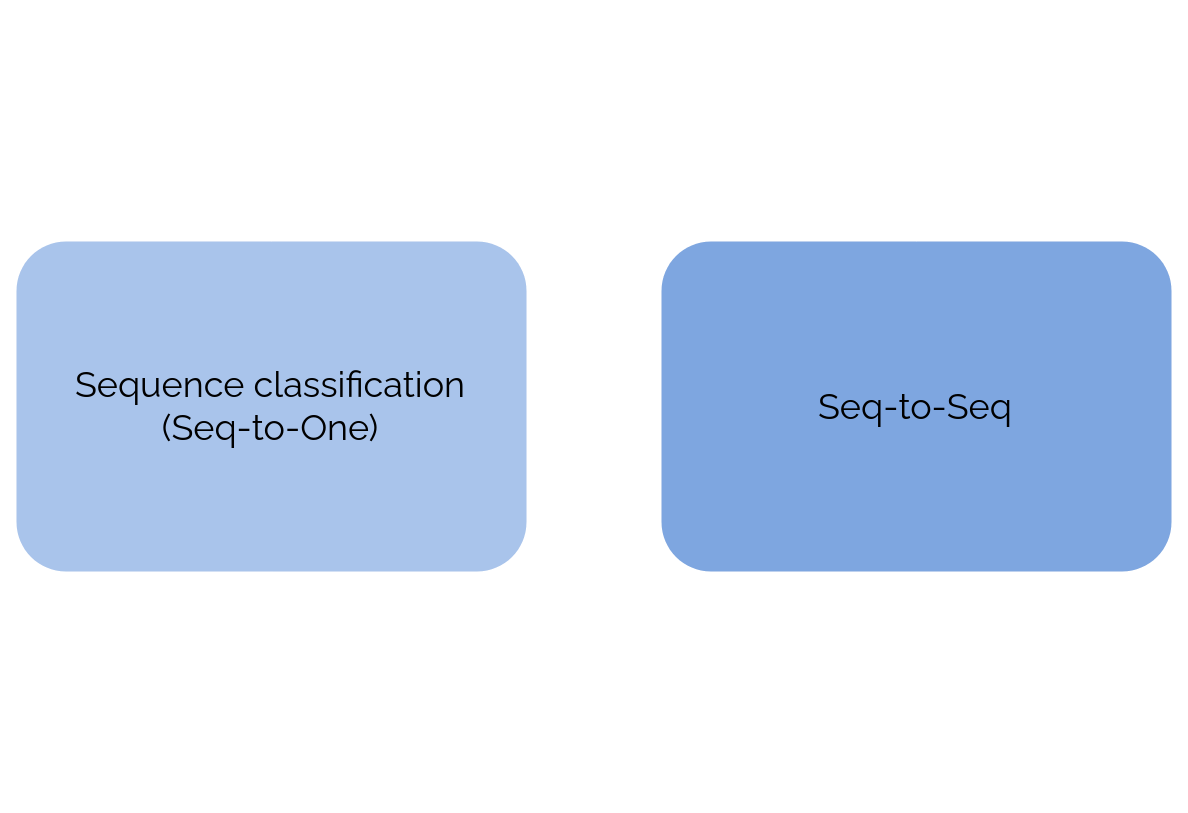
Seq-to-One vs. Seq-to-Seq
\(\to\) See the difference between the word embeddings of different sentences and the subtraction of the sentences' embeddings
First 150 values of real embeddings of dimension 1024
Embeddings
An embedding is the representation of some unit of the natural language in the form of a vector of real numbers.
For instance, an embedding could be a vector of 26 numbers where each of them represented the i-th letter of the alphabet and the quantity of the times such letter was found in a certain word.
However, embeddings tend to be more complex than this last example in which coin and icon would provide the same representation.
Recall that the vector represents the structure of the language we choose, not necessarily words: they could represent a letter, part of a word, a word or a whole sentence itself.
Although, the most common is for them to be a word or part of it.
\(\to\) Compare the differences between words and tokens with the same examples
First 150 values of real embeddings of dimension 1024
Tokens
In this Transformer architecture, each embedding represents a part of the word. The tokenization found depends on several aspects:
the algorithm of tokenization chosen, the frequency it has on the language and the encoding that is applied.
In addition, in this case, punctuation signs haver their own token (commas, apostrophes, etc) and a special one (<eos>) is used to indicate end of sentence (omitted in the plot). However, we
insist that this is characteristic of the chosen architecture and, thus, not a generalized or standard processing of the words.
One rapidly sees that the relationship between tokens and words is not linear, as it can be appreciated on the example.
Attention
The attention mechanism permits the network to identify which tokens are more related between them. In human terms, it is the
intuition that tells you that what is eaten is the carrot and who eats it is my mum. Mathematically, this is more abstract and harder to explain but
the base of all is the scaled dot-product attention and three specific vectors K, Q and V (shown on the right). We will dig into detail in Attention.
We will also see that the Transformer uses what is called multi-head attention and its types.
Scaled dot-product attention
Sinusoidal functions are usually used for positional encoding
Positional encoding
We have seen how the Neural Network identifies a word and how it relates their meanings, but how does it determine the order of the words?
Because obviously, saying 'My mum eats a carrot' is not the same as 'A carrot eats my mum'.
This is achieved thanks to what we call positional encoding, a vector of the same dimension as the embeddings that somehow contains information about the position
of the token within a sentence. Said vectors can be trained weights (optimized during training) or pre-defined functions that work well enough. In the Transformer,
the autors tried both methods using a mix of sinusoidal functions for the latter one, which they kept, as the results were pretty similar with both techniques.
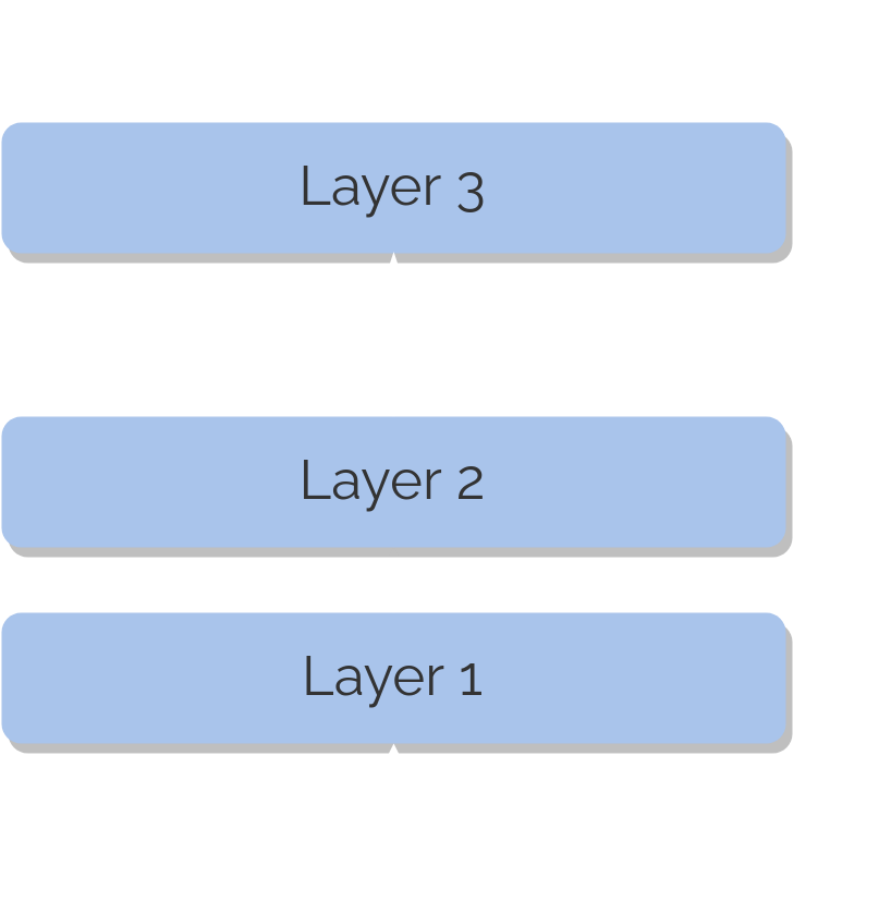
Residual connections
Also known as skip connections or skip-layer connections, are those steps in which a vector is copied and ommits one ore more layers and then it is used at the output of a posterior layer along with the output of such layer itself. There, it can be concatenated or added.
They are useful to avoid vanishing gradient problems and they act in such a way that the network does not 'forget' the past as easily, allowing the model to perform better.
As we will see in the architecture, the Transformer counts with several of them and are important to achieve the results it has. For instance,
positional information does not get lost or vanished due to the residual connections.
Diagram of skip connections
Architecture
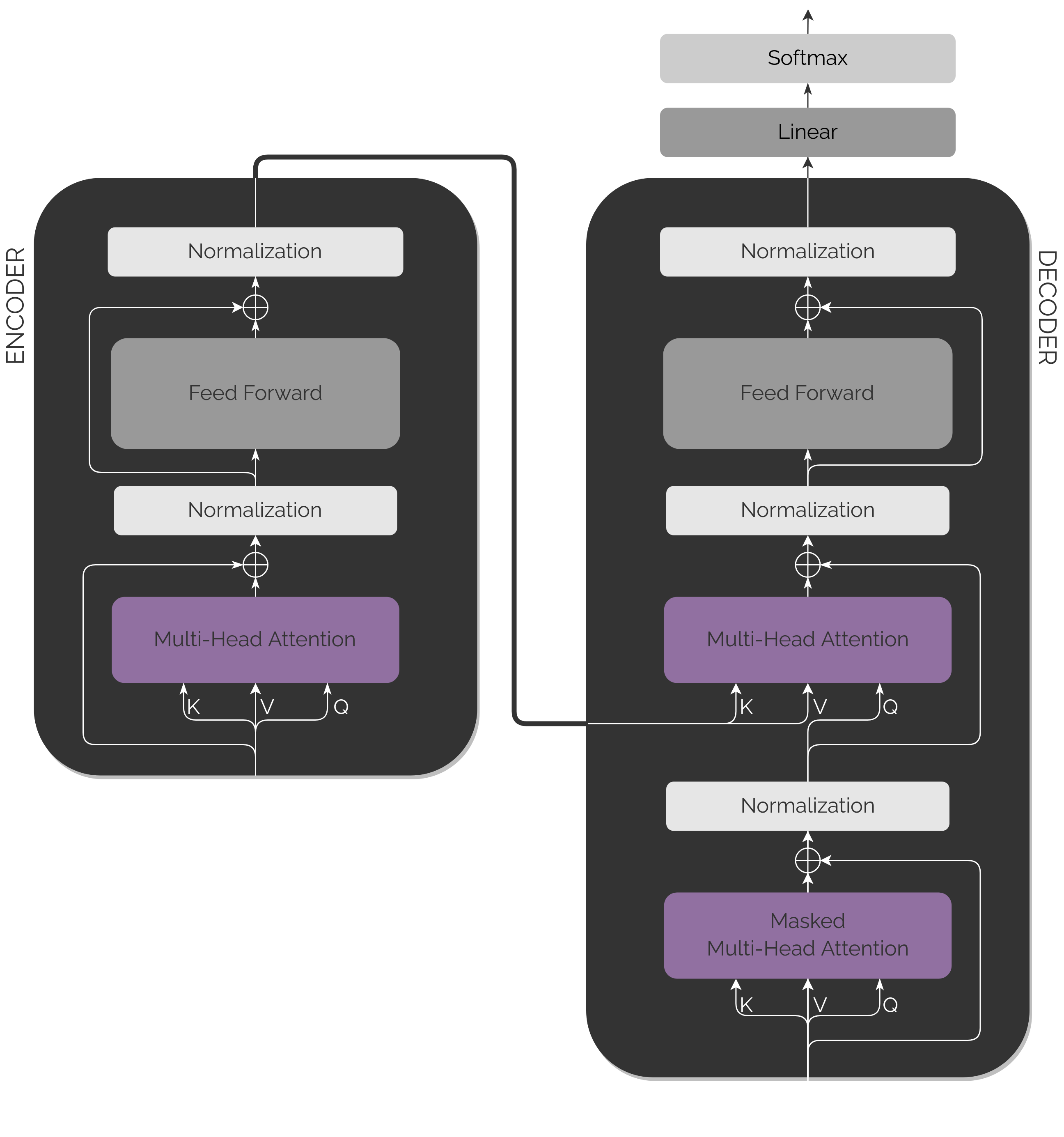
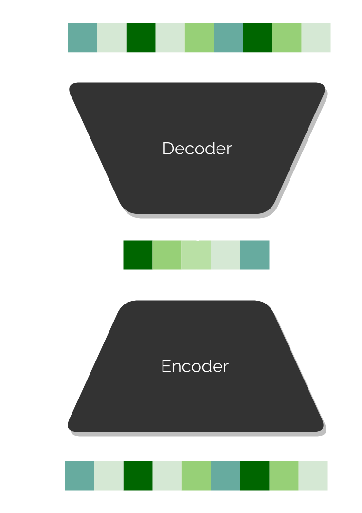
Encoder-Decoder
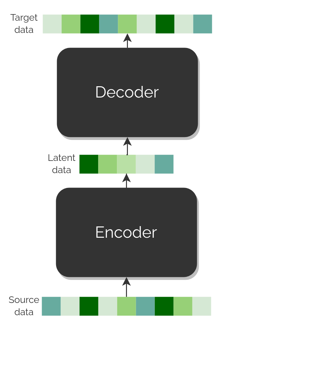
This type of architecture is a Neural Network that transforms the data using two modules: the Encoder and the Decoder.
The first one transforms the original data into an internal representation of it, which is sometimes referred as latent data or bottleneck in the literature.
The second one takes said representations and transform them into a desired target.
As for translation purposes, the Encoder works with the source language and the Decoder outputs the translation in the target language.
If the latent representations were generic enough, just by changing the Decoder one could train a Decoder that translated to any possible language.
Input set up
The input received in both parts, the Encoder and the Decoder, is an embedding that represents a token (recall, a part of a word).
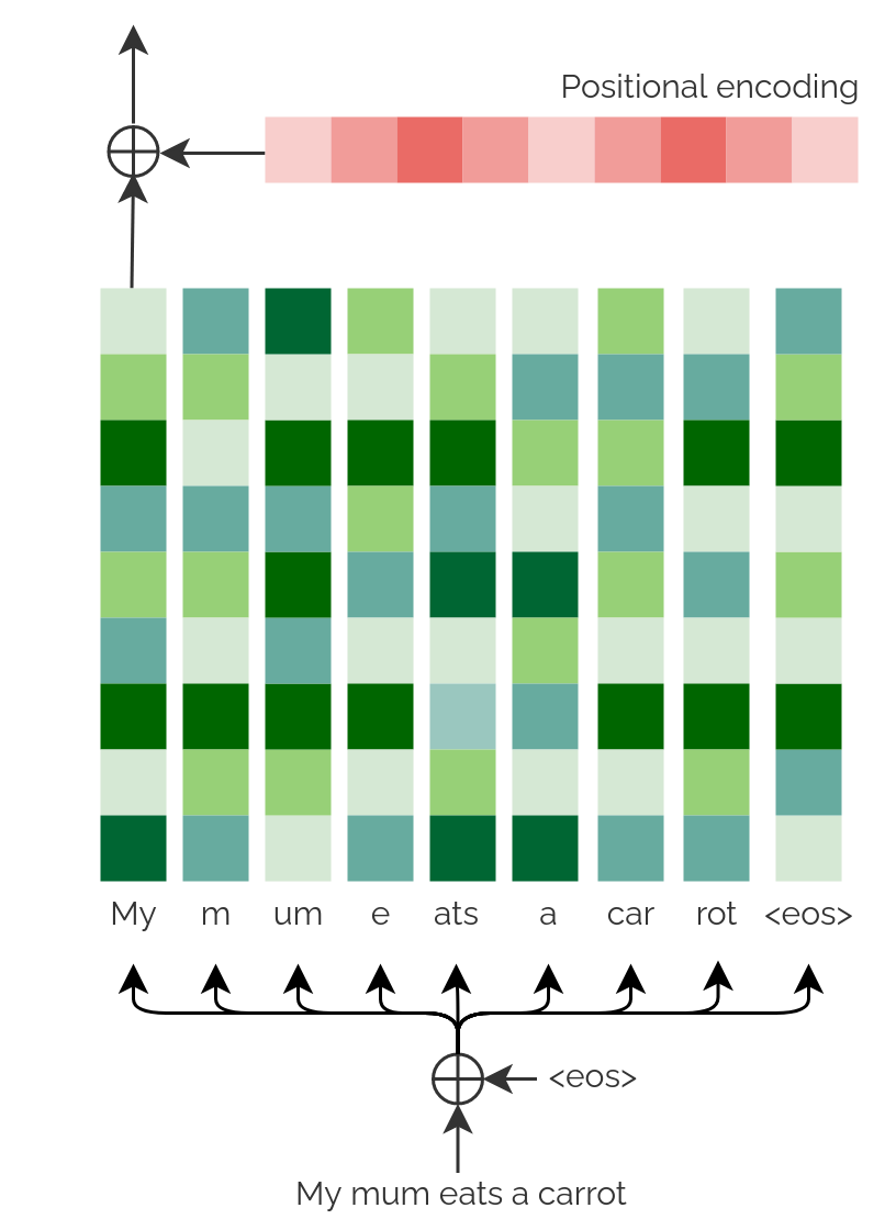
As this type of Neural Network is not recurrent (a type of network that does have a notion of temporality), it is added to each embedding
some specific weights that will determine the position each token has within the sentence, the positional encoding.
To exemplify, we input the English embeddings of the sentence in the Encoder. In the Decoder, we input the translated right shifted embedding of the Encoder input. In other words: the
last embedding we predicted in French.
To summarise, for each sentence we generate the tokens, we add the positional information and, then, they are ready to enter to the Encoder or the Decoder.
Positional Encoding
The weights of the positional encoding can be trained or determined by a function, typically a sinusoidal one. In the paper, said function is the following:
where \(pos\) is the position of the token in the sentence, \(d_{model}\) the dimension of the embeddings and \(i\) represents the position within the embedding.
In other words, in this particular case, to each embedding we add weights that come determined by the alternation of a sine and a cosine function (observable at your right) whose
objective is to state in which position a certain token is found.
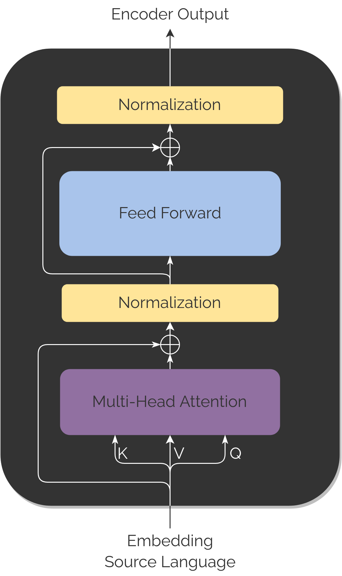
Encoder
After having the input embeddings prepared, the source language embeddings enter one by one to the Encoder, which will transform them into a
latent representation and will eventually go inside the Decoder.
It is worth mentioning that, unlike Recurrent Neural Networks, the input is just one vector and therefore we don't have the positional information
contained in any way, this is why positional encoding is needed.
Both modules contain mainly two blocks of layers: Feed Forward and Attention blocks. In addition, they also count with residual connections and normalization steps.
All of them are repeated in a total of N stacks (being N=6). That is, we have 6 times what we see in the diagrams.
This module is the most basic of the two.
Feed forward blocks
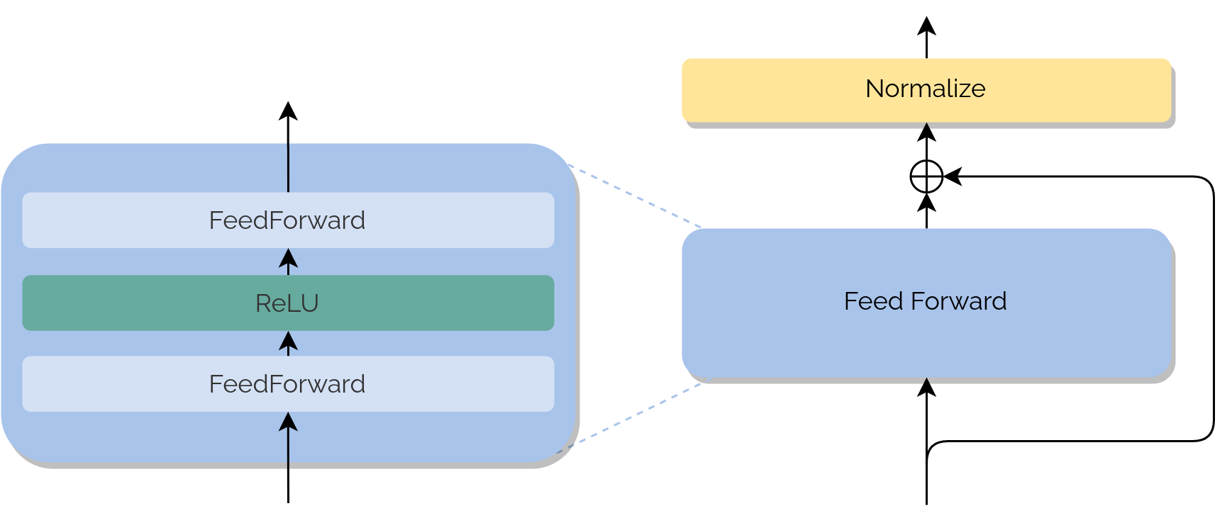
As we mentioned, in each module of the architecture, there can be found two main blocks, the first one is the Feed Forward. They are fully-connected Feed Forward Networks which
are applied to each position separately and identically. They consist of two layers with a ReLU activation in between and
the operations equate the behaviour of two convolutions of kernel size 1.
\(FFN(x) = max(0,xW_1+b_1)W_2+b_2\)
After each stack of layers, both in the Encoder and the Decoder, we have the addition of a skip connection and a normalization layer. This
helps the network to 'remember' the past and have small values inside the embeddings.
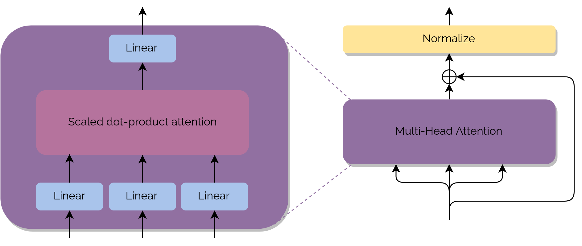
Attention blocks
The second main component inside the modules are the Attention blocks. In this paper, it is performed a simple
attention mechanism (scaled dot-product) that is combined with what it is called heads. This combination of techniques result
in what is known as Multi-Head Attention.
Each block of Attention consists of a linear layer, a scaled dot-product attention layer, a concatenation step and a final linear layer.
Also, one of the blocks (the first found in the Decoder) is referenced as Masked Multi-Head Attention. This is because we don't have all the information when predicting at that step,
so a mask is applied when training.
We will provide more detail in Attention.
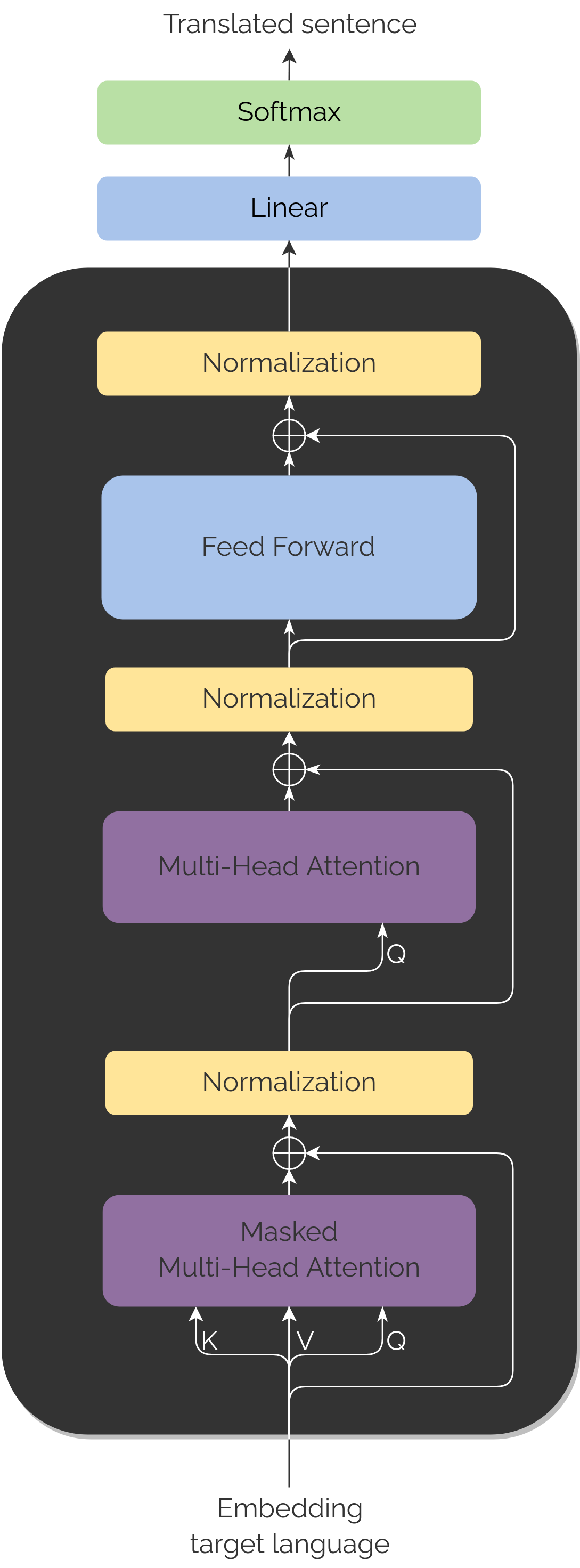
Decoder
The Decoder architecture is pretty similar to the previous one. In fact, we could say that, after the first Attention block and normalization, the architecture is basically the same.
However, the most noticeable differences are the inputs it has in the Attention blocks.
The first (at the beginning of the Decoder) is the target language embeddings shifted right (as we have already mentioned, the last predicted embedding).
The second one (in the middle of the module), passes as input the Encoder output and the Decoder embeddings that we have until that step.
Also, in here, we have two classes of Attention the first one being Masked Attention and the second a Encoder-Decoder Attention.
Notice that after the Decoder module we find two final layers, a linear layer and a softmax layer that will be in charge of choosing the most probable translation.
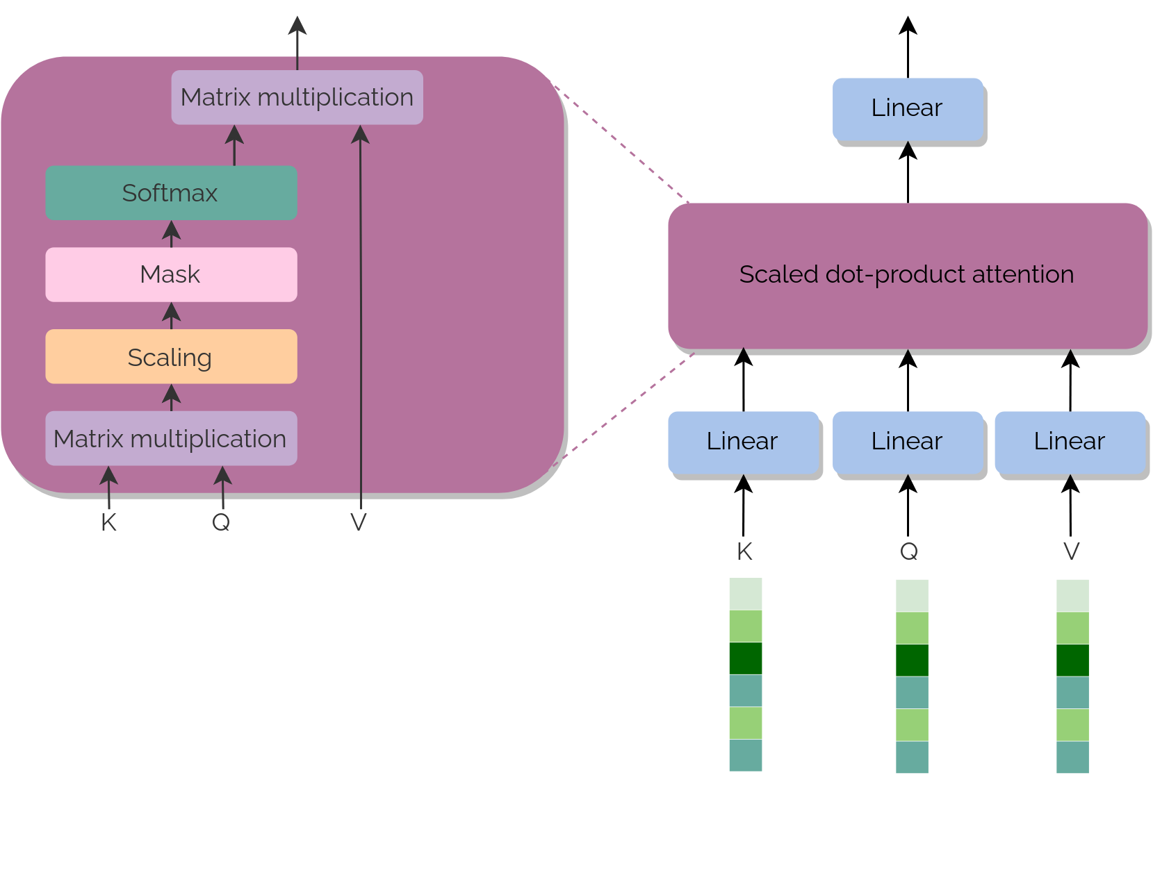
As we have introduced, attention is, in simple words, the mechanism that stablishes the relevance of a token in relationship with another.
To do so, it is necessary to
define the three components used: key (K), query (Q) and values (V). These are the vectors that we combine (map) in such a way that produce an output (also a vector) whose values define the mentioned relationships.
The output is computed as a weighted sum of the values (V), where the weight assigned to each of them is computed by a compatibility function of the query (Q) with the corresponding key (K).
In other words, K and Q are used to define some weights that will be used against V to define the importance between tokens.
We have three blocks in the Transformer architecture that perform this evaluation, but first let's describe better what an Attention block does.
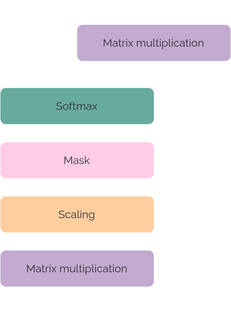
Attention blocks within Transformer architecture
Attention block diagram
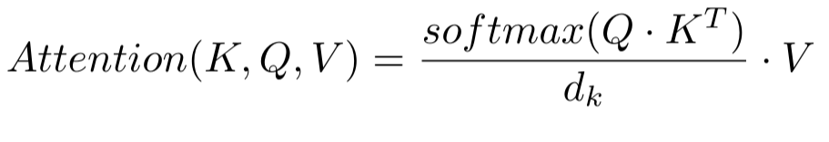
The attention itself is calculated as follows:
So each of the attention blocks perform this computation using the respective K, Q and V; which come from different sources according to the block they are found.
After performing the softmax, the result is scaled by \(d_k\) (the dimension of the embedding) and after it, it is multiplied by V. This way it is ensured that the vectors
we deal with are normalized at each step, a fact that is really helpful to avoid overflows and numeric problems.
Types
Having all this, one is capable to generate the Attention matrix. One may have a look at the architecure of the Transformer, from which we could
extract three attention matrices (as we have three blocks that compute it).
Self-Attention
The first block is found in the Encoder and uses the source language sembeddings as K, Q and V.
It somehow stablishes relationships among the sentence with itself in the source language, in our case, English.
Masked Self-Attention
The second block is found in the Decoder.
K, Q and V are the input of the Decoder which, remember, is the last output predicted (or the shifted right target).
It is called masked because, when we train, we mask the future data that we are not able to see when we predict (not having the data masked would imply that the network would see the future, hence it would be "cheating").
In other words, this Attention is computed with what we have so far in French.
Encoder-Decoder Attention
The third and last block is also found in the Decoder.
K and V are the output of the Encoder (thus, the tokens in the source language, English).
Q is the information we have of the Decoder up to that point, the shifted right outputs in French.
It is called Encoder-Decoder Attention due to the fact that combines the information of the Encoder (source language) and Decoder (target language), but
in terms of computations and structure it has no difference with the previous ones.
This might be the most interesting matrix of all three, as it shows the relationships of the tokens of the source and the target language.
Here we introduce real examples of the Self-Attention and Encoder-Decoder Attention matrices.
Heads
Up to this point, you might be wondering what exactly are heads in terms of Attention and what do they have to do in here.
Well, conceptually heads are not so willing to explain with an example because they are more like a helping 'feature' rather than a palpable thing itself.
Heads is the name assigned to the number of partitions we do to the input vectors (K, Q and V) in order to compute Attention separately. This allows the segmentation of the Attention
calculations and therefore the parallelization of this part of the model. Not only do we focus in smaller parts but also we permit them to be computed in a faster way,
hence a faster training.
So it is as simple as dividing the input vectors K, Q, and V into head parts. Then, they follow the same procedure as previously: a linear layer and the scale dot-product.
After it, we just concatenate the 'pieces' and pass through a last linear layer.
In the gif it can be observed the case where the number of heads is 3.
Training and usage
It's time to talk a little bit about the software part of the network. We are going to review, in general terms, which is the loss function, how the problem is
presented and some details that might be taken into account when building and training such Neural Network.
Loss function
The problem introduced is presented as a classification task in which the chosen 'class' will be the most probable word to be predicted.
The loss function that is minimized is known as the Cross Entropy Loss and is defined as follows:
Being \(k\) the total number of classes, \(y\) the target probabilities and \(\hat{y}\) the predicted probabilities.
As can be seen, it is generalized to any number of classes one may desire. It is also very useful and suitable for
classification problems, as it penalizes more the wrong predictions and rewards more the correct ones in comparison with what other losses would do.
Masks and prediction
We have already talked about masks. A mask is a special token (<MASK>) that replaces another token in a way that the Neural Network "does not take it into account". By this we mean that, if a token
is replaced by it, the Transformer will have no information about it, so it will work as if it was not there.
Masks are used during training in the first Decoder Attention Block as we have seen in the Architecture.
Similarly, masks are applied in many tasks of NLP, for instance, when training a next-word-prediction network where the future words hidden by the mask so that the network does not cheat.
Do It Yourself
If you wanted to train a Transformer architecture by yourself you would have two options:
Train from scratch with your own data and with your own coded architecture (or one imported from some library).
This is a tricky one as you would need to take into account: what dimensions to choose, how to perform the data processing (tokenization, deal with case sensitivity, etc),
choose hyperparameters, optimizers and more. Let's be honest, coding from scratch is not really common unless you have a special interest on doing all that by yourself. It is more common to take
the models available in different libraries and train with your own data, however if you don't have a big amount of data the best option is the next one.
You can take a pretrained network and fine-tune.
One of the advantages of the Transformers is that they are suitable for many tasks and contexts, typically for NLP, even though they can be used outside the language processing field.
Here, we have used the Transformer to translate from English to French. Needless to say, having a proper dataset in any other language would serve to train a translator to said language.
Besides, translation is not the only task that this type of architecture can perform.
Due to the outstanding results it provided, many different architectures and varieties arised since the publication of the original paper in 2017 and there are many open-source libraries that provide the code, data and
architecure to be able to fine-tune your own network.
Having all this information, training a Transformer architecture yields a whole world of opportunities:
Tasks
Next-sentence prediction
Question answering
Reading comprehension
Sentiment analysis
Paraphrasing
Applications
Machine translation
Document summarization
Document generation
Named entity recognition
Niological sequence analysis
Architectures
GPT-3
GPT-2
BERT
XLNet
RoBERTa
Distilled BERT
Details
In this section we provide further detail of some of the concepts already explained, more insight on some structures or elements that are specific for this network or any curiosity or feature that we consider worth mentioning.
We have learned what an Encoder-Decoder architecture is. In addition to this, it is interesting to have a look at the so-called Auto-Encoder.
This type of network is pretty famous and used as it is a simple but effective unsupervised method.
It consists of a network that is trained to predict exactly the same as it receives as input (weird right?). The trick of it is in the bottleneck (latent data) that is smaller than the initial and final dimension.
This way we train an Autoencoder that compresses the most relevant information and it remains condensed in a lowered-dimension than the original.
It is really helpful for compression, image segmentation, face recognition and others.
Special tokens are also a helpful feature to take into account. We have introduced the end-of-sentence tokens used in the paper. However, it is also usual
to find other tokens that do not directly reffer to a word: the beginning of sentence token <bos> (not used in this project),
punctuation signs tokens: <apos>, <,>, <.>, etc; and even a special token for unseen words <unk>.
Byte Pair Encoding (or digram coding) is a simple form of data compression.
It consists in replacing the most common pair of consecutive bytes of the data with a byte that does not occur within that data.
In NLP, it is a technique that can be applied as part of the preprocessing of the data and can help to reduce, memory-wise, the size
of the sets (training, validation and testing) considerably. This way, the training is speeded up while the quality is not seen affected.
But be aware, when predicting new data (using the network already trained) the BPE must be applied too!
Label Smoothing is a regularization technique that introduces noise for the labels / target. By doing this, we prevent the network to work with absolute zeroes,
hence saving it from computational issues. It is an easy, yet really helpful, technique to help the model generalize instead of overfitting by following really
strict patterns which, in the end, are not found in real life or when predicting never-seen-before targets.
As a matter of fact, it is only used in classification problems that use the cross-entropy function.
As we already know, Positional Encoding is what provides the network with the order information within the words or tokens. Quoting the authors:
"Since our model contains no recurrence and no convolution, in order for the model to make use of the order of the sequence,
we must inject some information about the relative or absolute position of the tokens in the sequence."
However, what do sinusoidal functions have to do with order?
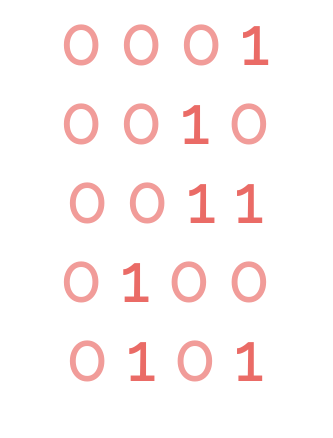
It is all related with the way bits change as they grow. If we observe the evolution of the bits when augmenting the numbers from one to five in binary, we observe the behaviour found in the right.
Somehow, every time we increase a number, this behaves at some level as a sinusoidal movement, here the reason why this type of function is appropiate for this task.
Therefore in the paper it is chosen a sine and a cosine function (shown below) that are alternated to simulate the change between numbers in a continuous form.
Sine and cosine components of PE
As this project intends to understand the overall ideas and intuitions behind the Transformer rather than digging into the details, we have avoided as much as possible
mentioning dimensions and specific numbers. Furthermore, they have many different factors that can affect them (the type of architecture, the structure of it, the way one may want to train the model,
the size of the data, the resources available, etc). However, there is one dimension that is interesting and useful in this type of task and does not always appear explained: the beam dimension.
We could define the beam dimension \((Be)\) as the hypothesis dimension we allow the model to investigate. As we already mentioned, the input of the Decoder is the last output and it can drag error.
That is why the network takes the top \(Be\) most probable tokens to be the translated, predicts each of the \(Be\) most probable next tokens and keeps, from the \(Be\) first hypothesized words, the one that provides less error. This is repeated at each step.
An example, if we want to translate our already known base sentence: My mum eats a carrot. We start the process, our beam dimension is \(Be = 2\), for the first word we hypothesize the translation to be ma and mon. The network will translate the following word taking into account
both articles: ma mère and mon mère and will conclude that, based on the error, ma is a better prediction.
This does not magically convert the network in the perfect translation machine, however it does lower the possibility of making a wrong prediction.
We have mentioned that after the Decoder, as latest step of the forward pass, we apply the softmax function. It is defined as:
The softmax function tries to replicate the behaviour of the maximum function. Why? Because this latter function is not differentiable and
it would not be possible for the network to propagate the gradients to be optimized (plainly, we couldn't train the network as it would not be able to update the weights).
For this reason a differentiable function that simulates the maximum is good enough, In addition, it is called soft as it still preserves a part of the non-maximum labels.
Activation functions determine if a neuron will be activated according to the value it has received. If this happens, the weights connected to the mentioned neuron will be updated during the backpropagation.
In this architecture we have seen the ReLU activation,
which is the abbreviation for Rectified Linear Unit. This function activates the neuron in case the input received is higher than \(0\), that is:
\( ReLU(x) = max(0, x) \)
However there are lots of different activation functions, each of them more suitable for certain contexts and tasks. Between the most common ones,
we can find the tangent activation function, sigmoid, linear... and many combinations or versions of it: Leaky ReLU, ELU, maxout, etc. The softmax function could also be included in this list.
The convolution is a type of operation usually performed in signal processing. It works with two functions: the main signal and
the kernel signal and it expresses how the shape of one is modified by the other. Mathematically, it is written as:
Being \(y(t)\) the convolution result, \(x(t)\) the signal and \(h(t)\) the kernel.
It has many uses and applications, even in Deep Learning. Long story short, Convolutional Neural Networks (CNNs) use the signal \(h(t) \)
as weights to be trained. Nowadays, they are one of the best networks to use in image and video recognition, image classification, etc. And as we have already
pointed out, the linear layer block weights act as a convolution of kernel size 1.
Learn more
The Artificial Intelligence universe is wide and it will soon be infinite, if you are interested in the topic, here you can find a bunch of resources that cover a variety of related work.
More state-of-the-art architectures, visualizing tools to understand them and social research upon ethics and bias inside NLP.